Why Power Dropdown

In-cell dropdown lists are an incredibly powerful Microsoft Excel feature, whether you are building complex workbooks where you or your users must select from sets of options or you are simply a user of such workbooks. They can save you from countless hours trying to spot a data entry error and help you build a lot more robust worksheets. If you are not using them yet, learn more about them here.

Creating an in-cell dropdown becomes easy after you try it a few times. Using it is also easy when it is short, meaning that your data validation list has only a few entries, let's say single-digit. With longer lists, it becomes harder. And as you get used to the feature and start finding it more and more useful, normally your data validation lists will start to grow. And with them, the frustration of you and your users will do the same, to the point that they may start thinking to switch back to typing again. Let's face it, selecting from a long list of predefined values can be as hard, or even harder, than typing the word. To be fair, Microsoft has thankfully improved the in-cell dropdown a lot lately: they added deduplication and a filter function, which limits the entries based on your text once you start typing. Power Dropdown does even more to improve in-cell dropdown lists:

• The list is displayed in a popup window, making it more user-friendly.
• The list automatically extends to the entire table column, if your data validation list is part of a table. Perhaps you have also experienced data validation lists not always extending when a table expands. Or a list that missed a cell or two when initially configured.
• You can choose to display additional text ("label"), next to the selectable value. Say, from another column of the table you are picking the valid values from. This can help the user pick the right option.
• The values are deduped, just like Excel now does by default. But if you added labels (see above), you can also take them into account while deduping.
• The popup window also includes a field which lets you filter the list. If you added labels, the filter also applies the filter to them.
• With the Premium version, you can also pre-define filters, which are applied to the data validation list before it is presented to you. Doing this is much more powerful but also more complex. It will be explained under the Advanced features section.
• And, finally, Power Dropdown still allows you to use the in-cell dropdown as you did before, as there can be cases where it remains the most convenient way to pick a value.

Quick start guide

You can install Power Dropdown from Microsoft Appsource: Power Dropdown Once the add-in is installed, it will appear as a new group under the "Data" ribbon in Microsoft Excel. Naturally, because this is where Data Validation also lives.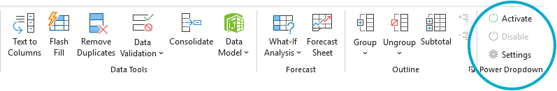

The easiest way to start using Power Dropdown is by clicking on the Activate button. This will activate the functionality using the default settings. We'll come to that later. While active, if you click once on an already selected cell (say near the middle) the data selection dialog box will appear on the screen:

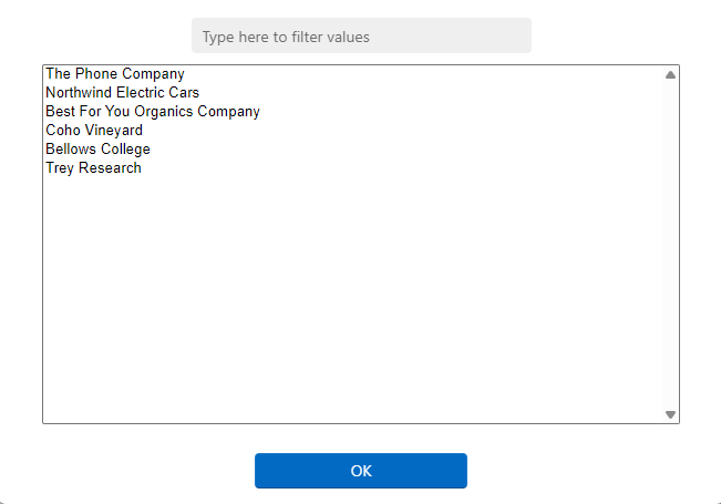
Start typing and the filter will start working, making the list shrink.
If you're down to a single value, just hit enter and it will be used.
If at any point you find that no good value is left (or no value at all), hit the F2 key and the filter will reset.
Hitting F4 will close the popup window.
You can also close the dialog by clicking on any Excel cell, outside the dialog.

You just experienced the most basic way to use Power Dropdown. Still the same as the in-cell dropdown, just a tad more convenient (at least I believe so). But wait, before you call it a day, let me teach you some one more thing: applying labels.

Appying labels

Labels are a great way to make selecting the right value easier. They can be used to add clarity about the value being chosen and also to enable filtering using text that is not part of the data validation list.
To add labels, you need to enter a JSON-formatted string right above the cell where you applied data validation. Or, if you applied data validation to a table, right above the title of your column.
You can also apply labels it using the Rule Editor, which is available in the task pane. the Rule Editor enters the JSON string in the right cell and can even keep it hidden, if the cell it belongs in is already used or if you prefer keeping our of the way.

If reading JSON makes you shiver, don't worry, it's not that hard. The Rule Editor makes it easier to write it, but the best way to explain is by using an example, so that's what we'll do. Let's imagine that you are picking data from this table: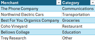

More specifically, you are picking data from the first column (Merchant), but you'd like to also have the second column (Merchant) displayed when choosing. The one thing you need to do, is add the following line above the cell with the dropdown list:

{"cml": {"labels": [{"offset": 1}]}}

Or this line, if your cells are within an Excel Table:

{"cml": {"labels": [{ "field": "Category"}]}}

Here is how it looks inside Excel:

And, by the way, you are not limited to a single label. You can add as many labels as you want, just by adding "fields" or "offsets" to the list inside the [] brackets, separated by commas. You know, inside the JSON array, like below:

Let's analyze the above briefly, for the unfamiliar with JSON:

• The outer {...} is denoting a JSON "object", with its "properties".
• "cml" is the name of the first property of object. Just a code so that Power Dropdown can be sure the text that follows should be interpreted as an instruction. Power Dropdown only uses this property, but there could be more.
• The {...} means that the the "cml" property of the object is actually an object itself.
• The first property of the "cml" object is called "labels". Because it will add labels to your data validation list. The [...] brackets mean that this property is an array, so it contains multiple properties one after the other.
• Inside the array you find objects one after the other, each object has a single property which can be named either "offset" or "label":
  • When it is an offset, the label will be whatever value is stored as many cells away from the data validation list as the offset indicates. Offsets can be positive, negative or even zero (although zero doesn't make much sense). The direction in which the offset is applied is vertical to the data validation list: for a vertical list, which I'd assume is the most common, the offset applies horizontally, spanning columns. For a horizontal list the offset applies vertically, spannign rows.
  • When it is a "field", which only works if the data validation list is inside a range formatted as a table, then the label will come from the table column which has the respective header.
• That's it! You can now build your labelled data validation lists. If you'd like to read more about the JSON format, you can find more information here:
  W3Schools: JSON - Introduction
  If you'd like to experiment with the advanced features, available in the Premium version, please keep on reading.

Configuration pane

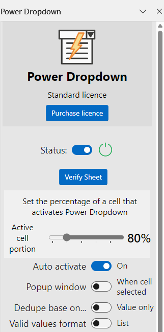
The configuration pane enables you to modify the way Power Dropdown behaves during use. You can also trigger some advanced functions, which will be explained later. The preferences are saved in the Excel file, so that when a user reopens it they will take effect. To open the configuration pane, click on the button, available on the Data ribbon. This will open the pane which looks similar to what is shown in the image on the right, which correcponds to the Premium version. Depending on the licence you have (Trial, Standard or Premium) the controls may differ. The following controls are available:

• On/Off button, labelled "Status": This allows you to switch Power Dropdown on and off. When in the off position, no popup window will occur.
• Verify sheet (Premium version only): When clicked, it checks whether the values selected in cells with data validation are consistent with filters configured in the validation rules. It can be useful when filters are configured and these are available only in the Premium version, which is why the button is displayed only then.
• Active cell portion: this controls the portion of a cell which, when clicked, will trigger the popup window to appear. By default it is set to the right 80% of the width of the cell, which means that, when Power Dropdown is active and the user clicks on the rightmost 80% of a cell with data validation, the popup window will appear. A user can choose to chenge this, from a minimum of 20% to a maximum of 100% at 20% increments. Reducing the active portion can be particularly useful when the popup is set to appear upon the first click on a cell (see Popup window option below), to avoid accidental popups.
• Auto activate: When set to the On state while Power Dropdown is also Active, it will cause Power Dropdown to activate automatically when the workbook is reopened. If you enable this option without Power Dropdown being Active, then the add-in will activate istelf once a user opens the task pane.
• Popup window: this affects the trigger for showing up the selection popup window. By default, (off position) the dialog will pop up only when clocking on an already selected cell. This is to avoid accidentally having the window pop up, which could end up being annoying. When set to the On position, the popup will appear as soon as the first click on the active cell portion of a cell with data validation occurs.
• Dedupe based on...: This controls whether option deduplication will consider the data validation list values only or their labels as well when deduplicating the entries. By default, only the values are considered, just like with the built-in in-cell drop down. A user can change the behaviour to take into account also the labels. This can be useful when, even though two options need to have the same entry, you want the user to be able to see more possible explanations. For example, you have a cell where the user needs to select whether a country is within the EU or not. For that, you have a list of countries in one column and in the next column whether the country is "EU" or "Non-EU". The data validation list only contains the values "EU"/"Non-EU" and you add a label to list all the possible countries, to help the user make the rigth choice by selecting a country. If the labels were ignored during deduplication, the validation list would only contain the first EU and the first Non-EU country, which would defeat the purpose. Hence, in such a case Power Dropdown should be set to Dedupe based on "Value & labels".
• Valid values format: This controls how the valid values are displayed in the popup. By default, they are displayed as a simple list with the labels separated by a dash (-). The alternative is to display the values and labels in a formatted table. This looks prettier and can be more user friendly, as the entries and labels are nicely separated in rows and columns and include the table row titles, if the data validation list is within a table. The downside is that it takes longer to process, especially if the list is long.

Advanced features

This section describes features included in the premium version only. When you start your trial period, all features are available. Once the trial period ends, you'll be limited to the features included in the version you are licenced to.

The following features are currently included in the Premium version:

• Validation list filtering
• Sheet verification function

Validation list filtering

This feature enables applying filters to the validation list already before the popup dialog is displayed (as opposed to applying a filter by typing text).
Filters can be very versatile and powerful once you get used to them. They become even more powerful when you apply filters to a series of cells with data validation that are related to each other, narrowing down the available options for each successive cell.

For example, let's say you start with a list of suppliers. Each supplier can supply multiple types of goods but not all. And each supplier can deliver to different countries. This ends up with too many combinations each time you try to choose a supplier.

Let's now imagine that we start with selecting a country where we want to deliver goods. Simple enough. Then we filter based on that country, to show only the goods that can be delivered in that country. And last, we filter the list of available suppliers based on both the goods and the country. This would make choosing the appropriate supplier much easier.

Let's see how we can apply filters using Power Dropdown. It is also done using a JSON object entered above the cell where we want to apply the filter, just like the label. The filter rule is slightly more complex, though. Here is an example:

    {"cml":{"filters":[
        {"filtertarget":{"field":"category"},"filtervalue":{"value":"groceries"}},
        {"filtertarget":{"offset":1},"filtervalue":{"offset":1},"operation":"eq"}}
    ]}
    

It may look a little scary, but it's not so hard to understand. Let's take it line by line.
The first line should look familiar if you read the part about labels earlier. It is the same "object", its first property being "cml" which is another object. And this is where we find the first difference: in the example about labels, the name of the property was "labels". Here it is "filters", because we are dealing with filters. Like the labels, it is an array of objects, starting with "[", which ends at the last line with the corresponding "]". The last line also marks the end of the "cml" and "filters" object.

The second line is the first filter in the array. The object has two properties: "filtertarget" and "filtervalue".
The property "filtertarget" defines the list of values which will be checked againt the filter. It is defined with respect to the data validation range, just like the label. If we take as an example the table on the right, and the validation list is the first column (Merchant), then "filtertarget" set to "category" means that the values in the "Category" column will be checked against the filter rule and only Merchants allowed by the filter will be included in the list.

The property "filtervalue" defines what the "filtertarget" will be compared against. In the example above, the first filter (second line) defines the "filtervalue" directly as a "value". This is taken literally, meaning that Merchants need to belong to the "groceries" category to be included. The "filtervalue" property, though, can be set to "field" or "offset", just like "labels" and "filtertarget". But be careful: the "field" or "offset" of "filtervalue" is defined with respect to the actual cell where data validation rule applies, the actual cell which will receive the selected value. This is different than the "labels" and the "filtertarget", both of which are defined with respect to the data validation range of cells.

The second example (third line) shows a slightly different approach: "filtertarget" and "filtervalue" are both defined using offsets. Remember, the "filtertarget" offset is defined based on the data validation list. If your data validation list is the first column of the same table as above (Merchant), then the "filtertarget" is, once again, Category. The difference now is that filtervalue can change depending on the content of a cell right next to the one you are selecting a value for. Just one cell to the right because offset is set to 1. So to get the same result as before, your cell would have to look like this: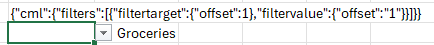

Notice that in this example only the second filter is applied and the "operation" property is missing. Now, if the value inside the cell on the right changes, the values displayed in the data selection pop-up will also change. The cell on the right could also have data validation, allowing a user to first choose the Category and then a Merchant matching that category. Imagine this also in a table, where each line correcponds to one acquisition, where the user first chooses the Category and then the Merchant. Then you could even have yet another list with the SKUs available from each Merchant, with descriptions for each SKU, allowing the user to pick from them. Powerful, right?

Finally, let's examine the last property: "operation". As the name implies, this controls how the filter is applied. The default is "eq", which stands for equal, and this is what was used in the second filter of the example. And that's why it could be ommitted later, in the Excel screenshot, without changin the result. When "operation" is set to "eq", only values where the "filtervalue" will match the respective value in "filtertarget" will be picked. Note that the comparison is case-insensitive for strings. This is the full set of operators that can be used:

• "eq": equal
• "ne": not equal
• "startswith": starts with the "filtervalue" character sequence
• "endswith": ends with the "filtervalue" character sequence
• "contains": contains the "filtervalue" character sequence
• "gt": greater than
• "lt": less than
• "ge": greater or equal
• "le": less or equal

Currently, an "AND" operator is assumed for all filter rules, meaning that all of them need to be true for the value to be included. This will be extended in the future, to enable even more versatile filters.

Finally, please note that you can also enter the entire JSON sequence with the label/filter rules in a single line without spaces, the only reason there were multiple lines in the example was to make explaining it easier. Therefore, rules could be entered as below, including both labels and filters and mixing multiple ways to reference (fields, offsets, values):

However, most likely you will find that using multiple lines will make it easier for you to format JSON without missing any commas/brackets. It might take a while to get used to but once you make it a habit you will see that the JSON format becomes intuitive and flexible.

Verify sheet button

Imagine that you have several (let's say a few tens at least) cells with in-cell drop down lists. You used Power Dropdown to apply filters to the validation lists. You cells depend on each other, in a way that changing one cell can affect several cells. And as you are working on your file, you decide to change the value of one of those "root" cells, which can affect many others. Excel data validation will be of no help, because all values will still be within the data validation list. You could click on each cell invididually, in which case Power Dropdown would warn you in case a value is invalid. But if you have many cells, this would be a really tedious process. And, following the motto of this web site, we should be lazy. The computer should to the work for us.

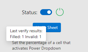"Verify Sheet" button to the rescue! As soon as you click on this buton, Excel will go through every cell which has data validation rules. It will also check the filters you have applied and compute the filtered list for every cell. Then, it will check against the value in the cell. If the value became invalid, it will add a comment to help you track it down. If only one value matches, it will fill it for you and the cell will flash green/yellow (but you don't really have to be looking). Once your computer is done checking the worksheet, the Verify Sheet button will become available again. If you hover on the button, you will get a summary of what it did, something like the image on the right.

Getting support

Feel free to email us if you need support using Power Dropdown.

Downloads

• Power Dropdown manifest
• Demo Excel file